Assignment 3
- Name: Aadam
- Class: INFO-B 518
- Assignment: 3
At a university, 13% of students smoke.
(a) Calculate the expected number of smokers in a random sample of 100 students from this university. (1 pt)
The expected number of smokers in a random sample of 100 students from this university is: \(E(x) = n \times p = 100 \times 0.13 = 13\).
(b) The university gym opens at 9 am on Saturday mornings. One Saturday morning at 8:55 am there are 27 students outside the gym waiting for it to open. Should you use the same approach from part (a) to calculate the expected number of smokers among these 27 students? (1 pt)
No, you should not use the same approach from part (a), because in part (a), the assumption is that the students are taken from a random sample from the university. Here, in this scenario, the students outside gym represent a specific group of students, not a random sample. That’s why we can’t use the same approach to calculate the expected number of smokers among them.
The average daily high temperature in June in LA is 77 F with a standard deviation of 5 F. Suppose that the temperatures in June closely follow a normal distribution.
(a) What is the probability of observing an 83 F temperature or higher in LA during a randomly chosen day in June? (1 pt)
The probability of observing at least an \(83 \degree\) F temperature is given by:
\[ \begin{aligned} Z = \frac{x - \mu}{\sigma} = \frac{83 - 77}{5} = 1.2 \\ P(T \leq 83) = P(Z \leq 1.2) \approx 0.885 \\ P(T \geq 83) = 1 - P(T \leq 83) = 1 - 0.885 = 0.115. \end{aligned} \] So, the probability of observing at least \(83 \degree\) F temperature in LA during a randomly chosen day in June is \(11.5\%\).
(b) How cold are the coldest 10% of the days during June in LA? (1 pt)
First, we need to find the z-score that corresponds to the 10th percentile (0.10) in the standard normal distribution table, which is approximately \(-1.28\). Now, we can use the z-score formula to find the temperature value (X): \[\begin{aligned}X &= \mu + \sigma \times z \\ &= 77 + 5 \times (-1.28) \\ &= 77 - 6.4 \\ &= 70.6\end{aligned}\] So, the coldest \(10\%\) of the days during June in LA would be around \(70.6\degree\) F or colder.
When patients receive blood transfusions, it is critical that the blood type of the donor is compatible with the patients, or else an immune system response will be triggered. For example, a patient with Type \(O-\)blood can only receive Type \(O-\) blood, but a patient with Type O+ blood can receive either Type O+ or Type O-. Furthermore, if a blood donor and recipient are of the same ethnic background, the chance of an adverse reaction may be reduced. According to a 10-year donor database, 0.37 of white, non-Hispanic donors are O+ and 0.08 are O-.
(a) Consider a random sample of 15 white, non-Hispanic donors. Calculate the expected value of individuals who could be a donor to a patient with Type O+ blood. With what standard deviation? (1 pt)
\[\begin{aligned}E(X) &= n \times (P(O+) + P(O-)) \\ &= 15 \times (0.37 + 0.08) \\ &= 15 \times 0.45 \\ &= 6.75. \end{aligned}\] The expected number of individuals who could be a donor to a patient with Type O+ blood is \(6.75\). Now, to find the standard deviation, we can use: \[\begin{aligned} \sigma &= \sqrt{n \times p \times (1 - p)} \\ &= \sqrt{15 \times 0.45 \times (1 - 0.45)} \\ &= \sqrt{6.75 \times 0.55} \\ &= \sqrt{3.7125} \\ &\approx 1.93 \end{aligned}\] So, the standard deviation is approximately \(1.93\).
(b) What is the probability that 3 or more of the people in this sample could donate blood to a patient with Type \(O-\) blood? (1 pt)
We can use the binomial probability formula to solve this exercise. As we know, that \(P(X \geq 3) = 1 - P(X \leq 3)\), so we can solve this exercise by computing the probabilities of \(X = 0, X = 1,\) and \(X = 2\), and subtract those from \(1\). Now: \[\begin{aligned} P(X = 0) = C(15, 0) \times (0.08)^0 \times (0.92)^{15} \approx 0.2863 \\ P(X = 1) = C(15, 1) \times (0.08)^1 \times (0.92)^{14} \approx 0.3734 \\ P(X = 2) = C(15, 2) \times (0.08)^2 \times (0.92)^{13} \approx 0.2273. \end{aligned}\] Now that we have calculated the probabilities of \(X = 1, 2, 3\), we can calculate the probability of \(P(X \geq 3)\) using: \[\begin{aligned} P(X \geq 3) &= 1 - P(X \leq 3) \\ &= 1 - (P(X = 0) + P(X = 1) + P(X = 2)) \\ &= 1 - (0.2863 + 0.3734 + 0.2273) \\ &= 1 - 0.887 \\ &\approx 0.113. \end{aligned}\] So, the probability that 3 or more people in this sample could donate blood to a patient with Type \(O-\) blood is approximately \(0.113\), or \(11.3\%\).
Approximately 12,500 stocks of Drosophila melanogaster flies are kept at The Bloomington Drosophila Stock Center for research purposes. A 2006 study examined how many stocks were infected with Wolbachia, an intracellular microbe that can manipulate host reproduction for its own benefit.
About 30% of stocks were identified as infected. Researchers working with infected stocks should be cautious of the potential confounding effects that Wolbachia infection may have on experiments. Consider a random sample of 250 stocks.
(a) Calculate the probability that exactly 60 stocks are infected. (0.5 pts)
\[\begin{aligned} P(X = k) &= {n \choose k} \cdot p^k \cdot (1-p)^{n - k} \\ P(X = 60) &= {250 \choose 60} \cdot (0.30)^{60} \cdot (0.70)^{190} \\ &= 0.006. \end{aligned}\]
(b) Calculate the probability that at most 60 stocks are infected. (0.5 pts)
Probability that at most 60 stocks are infected \((k \leq 60)\): \[\begin{aligned} P(X \leq 60) &= \sum_{i=0}^{60} C(250, i) \times (0.30)^i \times (0.70)^{250 - i} \\ &= 0.021. \end{aligned}\]
(c) Calculate the probability that at least 80 stocks are infected. (0.5 pts)
Probability that at least 80 stocks are infected \((k \geq 80)\): \[\begin{aligned} P(X \geq 80) &= 1 - P(X \leq 79) \\ & = 1 - (\sum_{i=0}^{79} C(250, i) \times (0.30)^i \times (0.70)^{250 - i}) \\ &= 1 - 0.7345 \\ &= 0.2655. \end{aligned}\]
(d) If a researcher wants to make sure that no more than 40% of the stocks used for an experiment are infected, does it seem reasonable to take a random sample of 250? (0.5 pts)
The expected number of infected stocks in a sample of 250 is given by: \[\begin{aligned} E(X) &= n \times p \\ &= 250 \times 0.30 \\ &= 75. \end{aligned}\] This means that we can expect approximately 75 stocks in a random sample of 250 to be infected. Now, if the researcher wants to make sure that no more than 40% of the stocks are infected, they would want the maximum number of infected stocks to be 40% of the sample size: \(250 \times 0.40 = 100\). Since the expected number of infected stocks in a sample of 250 is 75, which is less than 100, we can conclude that yes, it seems reasonable to take a random sample of 250 stocks to meet the researcher’s criterion of no more than 40% infected stocks in the experiment.
Consider the standard normal distribution with mean = 0 and standard deviation = 1.
(a) What is the probability that an outcome Z is greater than 2.60? (0.5 pts)
\[\begin{align*} P\left( {Z > 2.60} \right) &= 1 - P\left( {Z \le 2.60} \right)\\ &= 1 - \Phi \left( {2.60} \right)\\ &= 1 - 0.99534 \\ &= 0.00466 \end{align*}\]
(b) What is the probability that Z is less than 1.35? (0.5 pts)
\[\begin{align*} P\left( {Z < 1.35} \right) &= \Phi \left( {1.35} \right)\\ &= 0.91149 \end{align*}\]
(c) What is the probability that Z is between -1.70 and 3.10? (0.5 pts)
\[\begin{align*} P\left( { - 1.70 < Z < 3.10} \right) &= P\left( {Z < 3.10} \right) - P\left( {Z \le - 1.70} \right)\\ &= \Phi \left( {3.10} \right) - \Phi \left( { - 1.70} \right)\\ &= 0.9990 - 0.0446 \\ &= 0.9544 \end{align*}\]
(d) What value of Z cuts off the upper 15% of the distribution? (0.5 pts)
\[\begin{align*} P(Z \geq z) &= 0.15 \\ P (Z \leq z) &= 1 - 0.15 \\ P(Z \leq z) &= 0.85 \\ \phi(z) &= 0.85 \\ \phi(z) &= \phi(1.04) \\ z &= 1.04 \end{align*}\]
(e) What value of Z marks off the lower 20% of the distribution? (0.5 pts)
\[\begin{aligned} P(Z \leq z) &= 0.20 \\ \phi(z) &= 0.20 \\ \phi(z) &= \phi(-0.84) \\ z &= -0.84 \end{aligned}\]
In triathlons, it is common for racers to be placed into age and gender groups. The finishing times of men ages 30-34 have a mean of 4,313 seconds with a standard deviation of 583 seconds. The finishing times of the women ages 25-29 have a mean of 5,261 seconds with a standard deviation of 807 seconds. The distribution of finishing times for both groups is approximately normal. Note that a better performance corresponds to a faster finish.
(a) If a man of the 30-34 age group finishes the race in 4,948 seconds, what percent of the triathletes in the group did he finish faster than? (0.5 pts)
\[\begin{aligned} z &= \frac{X - \mu}{\sigma} \\ z &= \frac{4948 - 4313}{583} \\ z &\approx 1.089 \\ \phi(z) &= \phi(1.09) \\ \phi(z) &= 0.8621. \end{aligned}\] Now, to find the percent of triathletes that the man finished faster than, we need to subtract the calculated probabilities from \(1\), i.e., \(1 - 0.8621 = 0.1379\). So, he finished faster than about \(13.79\%\) of the triathletes in the men’s 30-34 age group.
(b) If a woman of the 25-29 age group finishes the race in 5,513 seconds, what percent of the triathletes in the group did she finish faster than? (0.5 pts)
\[\begin{aligned} z &= \frac{X - \mu}{\sigma} \\ z &= \frac{5513 - 5261}{807} \\ z &\approx 0.312 \\ \phi(z) &= \phi(0.312) \\ \phi(z) &= 0.6217. \end{aligned}\] Now, to find the percent of triathletes that the woman finished faster than, we need to subtract the calculated probabilities from \(1\), i.e., \(1 - 0.6217 = 0.3783\). So, she finished faster than about \(37.83\%\) of the triathletes in the women’s 25-29 age group.
(c) Calculate the cutoff time for the fastest 5% of athletes in the men’s group. (0.5 pts)
\[\begin{aligned} X &= \mu + \phi(0.05) \times \sigma \\ &= 4313 + (-1.644854) \times 583 \\ &\approx 3354.05. \end{aligned}\]
(d) Calculate the cutoff time for the slowest 10% of athletes in the women’s group. (0.5 pts)
\[\begin{aligned} X &= \mu + \phi(0.90) \times \sigma \\ &= 5261 + 1.281552 \times 807 \\ &\approx 6295.21. \end{aligned}\]
a. The final exam scores of 20 introductory statistics students are plotted below. Do these data appear to follow a normal distribution? Explain your reasoning. (1 pt)
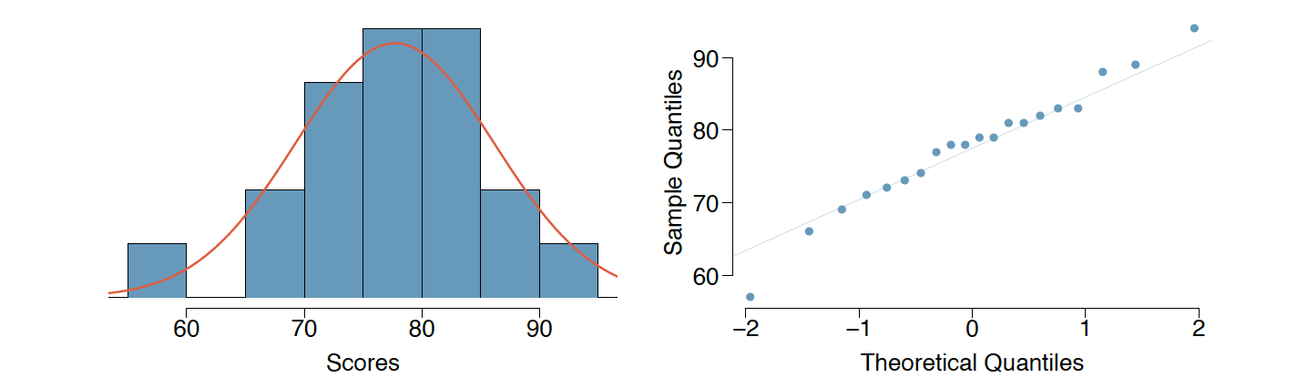
The distribution exhibits unimodality and symmetry, closely resembling a normal distribution as indicated by the overlaid normal curve. The points on the normal probability plot also exhibit a strong linear trend. Although a potential outlier is visible at the lower end in both graphs, it does not deviate significantly from the expected pattern. In summary, we can conclude that the distribution closely approximates a normal distribution.
b. The heights of 25 female college students are plotted below. Do these data appear to follow a normal distribution? Explain your reasoning. (1 pt)
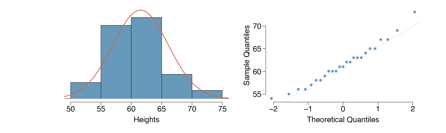
Based on the histogram and the Q-Q plot, the data seems to follow a normal distribution. We can see in the Q-Q plot that the data points tend to follow the line but with some deviation on both high and low ends, but looking at the data as a whole, we can conclude that it does appear to follow a normal distribution.
A very skilled court stenographer makes one typographical error (typo) per hour on average.
(a) What are the mean and the standard deviation of the number of typos this stenographer makes in an hour? (0.5 pts)
As we know, that the rate of distribution \(\lambda\) is given to be \(1\), so: \[\begin{aligned} \mu &= \lambda = 1 \\ \sigma &= \sqrt \lambda = \sqrt 1 = 1. \end{aligned}\]
(b) Calculate the probability that this stenographer makes at most 3 typos in a given hour. (0.5 pts)
Using the Poisson distribution formula: \[\begin{aligned} P(T \leq 3) &= \sum^3_{t=0} \frac{1^t \cdot e^1}{t!} = 0.981 \end{aligned}\]
(c) Calculate the probability that this stenographer makes at least 5 typos over 3 hours. (0.5 pts)
To calculate the probability that the stenographer makes at least 5 typos over 3 hours, we need to adjust the rate \((\lambda)\) for \(3\) hours.
The rate for 3 hours would be \(3 \times \lambda = 3 \times 1 = 3\).
Now, we want to find the probability of making at least \(5\) typos, which means \(P(T \geq 5)\). We can calculate this using the complement probability, where \(P(T \geq 5) = 1 - P(T < 5)\).
Using the Poisson distribution formula for \(t\) ranging from 0 to 4: \[P(T < 5) = \sum_{t=0}^{4} \frac{3^t \cdot e^{-3}}{t!} = 0.916.\] Now, to calculate the probability that this stenographer makes at least 5 typos over 3 hours, we need to subtract \(P(T \lt 5)\) from \(1\), which gives us \(1 - 0.916 = 0.084\). So, the probability that the stenographer makes at least 5 typos over 3 hours is \(8.4\%\)
A husband and wife both have brown eyes but carry genes that make it possible for their children to have brown eyes (probability 0.75), blue eyes (0.125), or green eyes (0.125).
(a) What is the probability the first blue-eyed child they have is their third child? Assume that the eye colors of the children are independent of each other. (1 pt) > \[\begin{aligned} P(X = 3) &= (1 - 0.125)^{3 - 1}(0.125) \\ &= (0.875)^2 (0.125) \\ &= 0.0957 \end{aligned}\]
(b) On average, how many children would such a pair of parents have before having a blue-eyed child? What is the standard deviation of the number of children they would expect to have until the first blue-eyed child? (1 pt)
\[\begin{aligned} \mu &= \frac{1}{P(X)} \\ &= \frac{1}{0.125} \\ &= 8. \\ \\ \sigma &= \sqrt{\frac{1 - P(X)}{P(X)^2}} \\ &= \sqrt{\frac{1 - 0.125}{(0.125)^2}} \\ &= \sqrt{\frac{0.875}{0.0156}} \\ &= \sqrt{56.089} \\ &= 7.48. \end{aligned}\] So, they can expect to have \(8\) children on average before having one with blue eyes, with a standard deviation of \(7.48\).
Let X represent the outcome from a roll of a fair six-sided die. Then, toss a fair coin X times and let Y denote the number of tails observed.
(a) Consider the joint probability table of X and Y. How many entries are in the table for the joint distribution of X and Y ? How many entries equal 0? (0.5 pts)
Given that \(1 \geq X \leq 6\) and \(0 \geq Y \le 6\), meaning that \(X\) can take on values between 1 and 6, while \(Y\) can take on values between 0 through 6. So, there are a total of 42 entries in the join probability matrix. The entries that equal \(0\) correspond to those entries where \(Y \gt X\), i.e., let’s suppose that \(Y = 3\) and \(X = 2\), then in this scenario it is impossible to get three tails when tossing a coin 2 times. So, the total number of entries that equal \(0\) would be: \(5 + 4 + 3 + 2 + 1 = 15\).
(b) Compute the joint probability P (X = 1; Y = 0). (0.5 pts)
\[P(X = 1; Y = 0) = (1/6)(1/2) = 1/12.\]
(c) Compute the joint probability P (X = 1; Y = 2). (0.5 pts)
As discussed in
(a), this scenario is impossible. This scenario refers to the case when the die rolls \(1\) and \(2\) tails are observed from \(1\) flip of the coin, which is improbable. So, it has a probability of \(0\).
(d) Compute the joint probability P (X = 6; Y = 3). (0.5 pts)
This probability can be obtained by multiplying the probability of getting a 6 on the die, with the probability of getting three tails when tossing a coin six times. The probability of getting three tails in a sequence of six coin tosses can be calculated using the binomial probability formula. So, the join probability is: \[\begin{aligned} P(X = 6; Y = 3) &= \frac{1}{6} \times \left( {6 \choose 3} \left( \frac{1}{2} \right)^3 \left( \frac{1}{2} \right)^{6-3} \right) \\ &= \frac{1}{6} \times \left( 20 \times \frac{1}{8} \times \frac{1}{8} \right) \\ &= \frac{1}{6} \times 0.3125 \\ &= 0.0521. \end{aligned}\]